Sunk Costs

Forecasting the Economic Impact of Sea Level Rise on Miami

This project is currently under development.

The site is available as a common reference, however it is worth noting that it is currently unfinished. The site, and the model, will continue to be developed in the near term.

You can press Cmd + K or Ctrl + K to open the quick search bar if you want to find something specific across the site.

All data visualizations on this site are interactive. Double click a plot to reset to the original zoom.

Sunshade Project Context

The focus of this report is the economic forecast, however the analysis was performed to contrast the cost of losing Miami to sea level rise with the cost of deploying a space based sunshade for geoengineering purposes. The project proposal was presented in 2022 at the New Worlds space conference in Austin. A modified document.slides.earthshade.pdf for the proposal is included on this site.

Issues & Continuous Development

This analysis and model are subject to change. If you find an issue with the methodology or have a suggestion for an improvement, please submit it in the GitHub repository - either in the issues or discussions sections depending the type of feedback you are submitting.

---

Overview

The objective of this project is to create a simple model that can forecast the economic cost of sea level rise (SLR) on the City of Miami by the year 2150. This report provides an (ideally) engaging introduction to the model, along with secondary analyses not included in the primary model.

It is important to point out that this model attempts to forecast cost in the absence of human intervention. It seems reasonable to expect this will occur as costs begin to materialize.

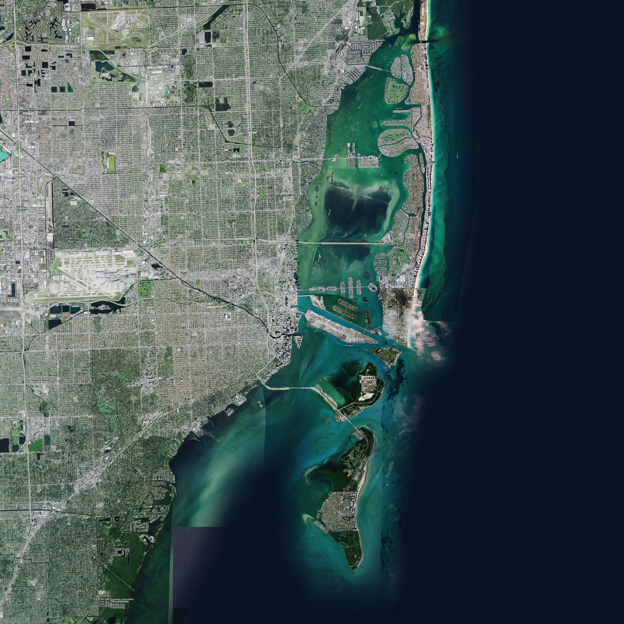
Before we begin, let's establish the geographic bounds of the region we will evaluate. (1) We'll refer to this as the "Analysis Area" or AA for short.

1. Coordinates for the bounding box are included below.

   coordinates = {
       "top_left": {
           "lat": 25.920,
           "lon": -80.350,
       },
       "bottom_right": {
           "lat": 25.655,
           "lon": -80.060,
       },
   }
   

Satellite Image

Summary

We recognize that not everyone will have time to read the full report. Accordingly, forecasts of economic impact for best case (low cost), baseline (medium cost), and worst case (high cost) scenarios by the year 2100 are included below. (1) Currently, only the best and worst case are included. Also note that the videos show SLR at 2100, but the final model will go out to 2150. Also, note that these are currently ballpark figures and will be adjusted as the model is streamlined.

1. Note that these dollar figures are almost certainly incorrect, and also not actually the figures the model returns, but rather figures derived from the output of the model. Regardless, they are included on the basis that decisive predictions - though virtually always wrong (or if right, by chance) - do have a certain psychological appeal.

~50 Billion

~300 Billion

Visualization will be included in complete version

~900 Billion

---

Introduction

Debatably, objectively quantifying cost is impossible on an epistemological level. Regardless, we will make an attempt. To do so, we must first establish the "factors" we will consider - Locke's life, liberty, and property might be a good place to start. We'll address these factors in the order of increasing complexity of model representation.

Economic Value Subjectivity

Tangible vs. Intangible Assets

When we speak of the economic impacts of sea level rise, we often first consider tangible assets – properties, infrastructure, and physical goods that can be directly measured in monetary terms. But how do we categorize and put a value on intangible assets impacted by SLR?

A renowned artist has painted a mural on a building's exterior wall in a coastal district of Miami. This mural becomes a significant cultural and tourist attraction. Over the years, its intangible value in terms of cultural identity and tourism appeal grows exponentially. Now, due to SLR, there's a real threat of the building being submerged or destroyed. How do we quantify the loss of this mural?

If we look at it in terms of the artist's fee and the material costs, the monetary value might be relatively low. However, when factoring in its cultural significance, the lost potential tourism revenue, and its irreplaceability, the value becomes more nebulous.

Collective vs. Individual Loss

Economic impacts can be felt at both individual and collective levels. For instance:

A family-owned restaurant that has been operating for decades at Miami's seafront might face bankruptcy due to SLR causing frequent flooding in the area. On a macro level, the economic loss from this single restaurant might seem insignificant when talking about the entire city's economy. But for the family running it, it's their livelihood, heritage, and perhaps a significant part of their identity.

Is it justifiable to weigh the city's overall economic health over the devastating loss of a single family's livelihood? It's subjective and varies based on who you ask.

Direct vs. Indirect Monetary Loss

While direct losses like property damage due to SLR are (relatively) straightforward to quantify, indirect losses can be nebulous.

Due to constant threats of flooding, insurance premiums for properties in Miami might skyrocket. This can lead to reduced property values and, subsequently, reduced property tax revenues for the city. The cascading effect might also mean businesses relocating, leading to job losses and reduced economic activity in affected areas.

While we can quantify the immediate losses due to property damage, how do we adequately measure the long-term economic ripple effects of such events?

Sea Level

Before we go into the details of quantifying the economic impact, lets' first focus on sea level rise.

Historical Global Sea Level

To provide context, let's take a short detour into historical sea level trends on planet Earth. We'll start by looking at the global sea level trend over the last few decades using data from the Jason Satellite Missions. The data used for this visualization can be downloaded here - we're using the set with seasonal signals removed. (1)

1. This is the data with seasonal signals removed. The difference between datasets with "seasonal signals retained" and "seasonal signals removed" pertains to the treatment of seasonal variations in the data. In the context of sea level data, seasonal signals could include variations caused by thermal expansion, melting glaciers, and other factors that follow a seasonal pattern.

   • Seasonal Signals Retained: This dataset includes the seasonal variations. It reflects the actual measurements taken over time, inclusive of all the fluctuations that occur on a seasonal basis. It can be useful for understanding how different factors contribute to sea level changes over the course of a year.
   • Seasonal Signals Removed: This dataset has been adjusted to remove the seasonal variations, providing a smoother trend over time. By removing the seasonal signals, it's easier to observe long-term trends and compare data across different time periods without the noise of seasonal fluctuations.

It is of course technically possible that the sea level has been rising for some time. For the sake of curiousity let's zoom out and look at the last few millenia. We'll use data produced by Kopp et al. from this research paper on historical global mean sea level. (1) The dataset can be downloaded here. (2)

1. The 1s column representing confidence is dropped in this visualization to simplify the output. From the paper:

   Each database entry includes reconstructed RSL, RSL error, age, and age error. For regional reconstructions produced from multiple sites (e.g., ref. 5), we treated each site independently. Where we used publications that previously compiled RSL reconstructions (e.g., refs. 37 and 45), the results were used as presented in the compilation. RSL error was assumed to be a range unless the original publication explicitly stated otherwise or if the reconstruction was generated using a transfer function and a Random Mean SE Standard Error of Prediction was reported, in which case this was treated as a range.

2. Also, the industrial revolution start date reference taken from wikipedia page on the industrial revolution.

So far we've only found that the sea level has been rising - but will it continue to rise?

Future Global Sea Level

Given the immense complexity and myriad factors influencing the sea level, creating a climatic model to forecast future sea level rise is beyond our capabilities. (1)

1. Interactions between the atmosphere, hydrosphere, geosphere, and even biosphere need to be accounted for, with each having its own set of variables and sub-variables that intertwine in ways that are not always predictable. Small changes in one factor, such as volcanic activity, solar radiation, or even human emissions of greenhouse gases, can have cascading effects throughout the system. What's more, feedback loops – both positive and negative – can amplify or dampen these effects in unforeseen ways.

Thankfully, smarter folks than us have already done this, namely: the IPCC. Of course, predicting the future is difficult if not impossible, so the IPCC provides us with a number of different scenarios in the form of SSPs (previously known as RCPs) through which we can evaluate the possible futures we face. We'll be focusing on SSP 126, 245, and 585, which we'll refer to as the 'best', 'medium', and 'worst' case scenarios.

SSP	Scenario	Scenario Details
119	Best	CO2 emissions cut to net zero around 2050.
245	Medium	CO2 emissions around current levels until 2050, then falling but not reaching net zero by 2100.
585	Worst	CO2 emissions triple by 2075.

The data we will use to model the different scenarios comes from the IPCC AR6 report. It can be downloaded here. (1)

1. It's important to note that our model \(M_1\) (for cost) uses a model \(M_2\) (for sea level rise) that is fit to the output of a model \(M_3\) (that the IPCC created). More details on the \(M_2\) to \(M_3\) process can be found in this informal jupyter notebook documenting the process.

The IPCC global sea level projections data is split into two confidence levels: 'low' and 'medium'. We'll be using only the medium confidence level. Without going into the details, we can use the IPCC data to model the probability density of given sea levels in each scenario out to the year 2150. An example for the SSP 245 scenario at the year 2100 is included below.

If we want to get the probability that the sea level will be in a certain range (1) we can get the area under the curve between two intervals.

1. Again mind you, for this scenario, confidence level, and specific year, from the IPCC estimates, from the skewed normal distribution I fit to the IPCC estimates.

If we display the probability distributions for each decade, for each scenario, we get the following graphs.

It is easier to see how the probability distributions differ if we graph them against each other on the same plot. This can become visually crowded quite quickly, however, so we've included just scenario 126 and 585 below, from 2080 onwards. Remember that these visualizations are interactive, so you can click and drag the graph to rotate it and get a better view.

Sections below are a work-in-progress.

Regional Differences

Introduction

The Big SIP

Property

We'll assume that the loss of property due to SLR has a negative economic impact.

Applying to Model

Property Value

Starting with property cost, we'll take the following premises as true. (1)

1. In a number of cases we will assume potentially false premises to be true, as not doing this would significantly increase the complexity of the model, and accordingly is out of scope. We will attempt to point out limitations and issues with each premise though. Then, if the reader would like to replicate, modify, or improve the code associated with the model, they have a headstart on some of the stuff that could be addressed.

If an area is inundated with sea water, we consider the property in that area lost.

If an instance of property is lost, we consider the market value of the property lost to be a cost.

Already, an issue presents itself. Namely, when we are considering the market value of the lost property, at what point it time should we assess its value?

It seems reasonable to assume that when the property has already been lost to sea level rise, the property value would be $0. Furthermore, once it becomes evident to the market that a property will be lost to SLR in the short term, we would also expect that the the market value would converge to zero.

As such, we should not assess the lost market value by looking at the market value, but rather by looking at what the market value would be in the absence of SLR, comparing it to the market value in the presence of SLR (and specifically, various potential SLR scenarios), and taking the difference between the two.

Unfortunately, this is an unpredictable and dynamic system.

Life

Liberty