AR6 SLP Model Methodology¶

This page documents the methodology used to produce the AR6 sea level projection sub-models from the IPCC data. It is included because I'm not entirely sure what I did is statistically valid, so I thought it would be a good idea to document the process so any flaws I introduced can be pointed out.

In [77]:

import sys
import pandas as pd
import numpy as np
import plotly.graph_objects as go
from copy import deepcopy
from loguru import logger as l
from scipy import integrate
from scipy.stats import skewnorm, kstest
from numpy.typing import ArrayLike
from sunkcosts.model.ar6 import SLP
from sunkcosts.plotly import MINIMAL

_ = l.remove()
_ = l.add(
    sys.stdout, colorize=True, format="[<green>{level}</green>] <cyan>{message}</cyan>"
)

import sys import pandas as pd import numpy as np import plotly.graph_objects as go from copy import deepcopy from loguru import logger as l from scipy import integrate from scipy.stats import skewnorm, kstest from numpy.typing import ArrayLike from sunkcosts.model.ar6 import SLP from sunkcosts.plotly import MINIMAL _ = l.remove() _ = l.add( sys.stdout, colorize=True, format="[{level}] {message}" )

First, I'll quickly note that the original data was in a NetCDF format that was a pain to work with. Accordingly, I built a dataclass for working with the data, which we'll use here.

More information on the data conversion process, and the .ssp (ie: JSON) files that the dataclass fetches the loaded data from can be found in this repository.

We'll start by loading the medium confidence SLP 245 scenario.

In [2]:

slp = SLP.load(confidence="medium", scenario="245")

slp = SLP.load(confidence="medium", scenario="245")

We can view the scenario data as a dataframe.

In [3]:

slp.data.table

slp.data.table

Out[3]:

	0.000	0.001	0.005	0.010	0.020	0.030	0.040	0.050	0.060	0.070	...	0.930	0.940	0.950	0.960	0.970	0.980	0.990	0.995	0.999	1.000
2020	28	31	34	35	36	37	38	39	39	40	...	70	72	73	76	79	85	97	112	138	165
2030	44	57	62	65	67	69	71	72	73	74	...	134	138	141	146	153	163	187	213	267	318
2040	55	84	92	96	101	104	107	108	110	111	...	207	213	219	227	238	255	296	336	408	490
2050	107	121	134	140	147	151	154	157	159	161	...	303	310	318	330	346	374	428	492	589	714
2060	80	148	166	174	183	189	193	197	200	202	...	397	407	419	434	457	497	570	646	789	947
2070	83	156	200	212	224	230	237	242	245	249	...	509	521	537	556	587	638	722	825	1005	1207
2080	75	175	220	243	262	273	280	287	291	295	...	627	643	663	690	730	789	904	1015	1244	1544
2090	84	177	256	273	295	308	318	326	333	340	...	753	771	795	827	875	959	1092	1230	1509	1907
2100	106	175	277	305	332	351	362	371	380	387	...	888	917	946	982	1038	1126	1283	1444	1777	2252
2110	207	285	324	342	366	379	391	400	409	416	...	1030	1055	1086	1140	1205	1300	1496	1684	2035	2618
2120	224	311	356	376	401	418	431	442	452	459	...	1161	1189	1227	1285	1359	1469	1691	1896	2303	2984
2130	238	335	386	408	436	455	470	482	493	502	...	1293	1322	1367	1428	1513	1638	1885	2104	2569	3345
2140	254	357	415	440	469	492	508	522	534	543	...	1424	1456	1506	1572	1668	1803	2079	2315	2833	3707
2150	269	378	443	470	502	528	545	560	572	584	...	1552	1590	1643	1713	1817	1970	2269	2518	3089	4068

14 rows × 107 columns

A quick explanation of what this dataset is:

• Each row represents the sea level projections for a year.
• Each column represents a probability quantile.
• Each cell represents a sea level change in millimeters.

Sea Level Change

The sea level change is measured since the AR6 reference period, a quote is included below from the FACTS_confidence_output_file_readme that can be found in the original dataset.

The level of sea-level change since the AR6 reference period.

Honestly, I'm not sure what the AR6 reference period was exactly, so I kind of overlooked that. That is definitely a glaring limitation of this model/analysis.

Correction, it is:

relative to a baseline of 1995–2014

From: IPCC AR6 report, page 1302, table 9.9 commentary

Probability Quantile

I'm not entirely sure I understood the quantiles correctly. The wikipedia page for quantiles states that:

There is one fewer quantile than the number of groups created.

But this is not the case in this dataset, where there are 107 quantiles and 107 sea level change values.

The aforementioned FACTS_readme PDF says the following, but I still wasn't sure.

Quantiles of the probability box of the sea-level change variable. 107 quantiles are available, including 0.0 to 1.0 in 0.01 increments and a few key quantile values (i.e. 0.995, 0.999, etc.). Multiply the quantiles by 100 to get the equivalent percentile values.

What was initially unclear to me was whether the quantiles are the probability that a sea level change will be manifested, by a year, or they are implicitly probability buckets, or something else. At any rate, I asked ChatGPT and got the following answer:

In statistics, a quantile is a location in a set of data that divides the data into groups with the same number of values below and above it. Quantiles at 0 represent the minimum value in the dataset, while quantiles at 1 represent the maximum value. If this dataset is describing sea level changes, each quantile value would correspond to a different scenario of sea level change. In your DataFrame, the numbers along the top (0.000, 0.001, 0.005...etc.) are the quantiles. The numbers in the rows are the sea-level changes for those quantiles in that particular year. So, for example, the value of the cell in the 2030 row at the 0.001 quantile is 40 millimeters. This means that, in the 2030 scenario, there is a 0.1% probability that the sea level will rise 40 millimeters or less. Here's another example. In 2040, the value in the 0.030 quantile is 93 millimeters. This means that, in the 2040 scenario, there is a 3% probability that the sea level will rise 93 millimeters or less. These elements are cumulative: a quantile of 0.030 means that 3% of the total outcomes fall below this value.

This seemed to more or less make sense, because if we graph the quantiles for a year the graph matches loosely what we would expect from this description.

The data from 2030 is graphed below.

In [4]:

data = slp.data.table.loc[2030].reset_index()
ycol, xcol = ["quantile", "mm"]
data.columns = [ycol, xcol]
quantiles = np.array(data["quantile"].tolist())
sealevel = np.array(data["mm"].tolist())

fig = go.Figure()

fig.add_trace(
    go.Scatter(x=sealevel, y=quantiles, mode="lines+markers", name="lines+markers")
)

fig.update_layout(
    title=f"{ycol} vs. {xcol}",
    title_x=0.5,
    template=MINIMAL,
    xaxis_title=xcol,
    yaxis_title=ycol,
)
fig.update_layout(title_x=0.5, height=600)
fig.show(renderer="notebook")

data = slp.data.table.loc[2030].reset_index() ycol, xcol = ["quantile", "mm"] data.columns = [ycol, xcol] quantiles = np.array(data["quantile"].tolist()) sealevel = np.array(data["mm"].tolist()) fig = go.Figure() fig.add_trace( go.Scatter(x=sealevel, y=quantiles, mode="lines+markers", name="lines+markers") ) fig.update_layout( title=f"{ycol} vs. {xcol}", title_x=0.5, template=MINIMAL, xaxis_title=xcol, yaxis_title=ycol, ) fig.update_layout(title_x=0.5, height=600) fig.show(renderer="notebook")

This was somewhat confusing to me, but I think the way to interpret it is to say that the quantile is the probability the sea level will rise less than a given value. So, for instance, the 0.1 quantile (10% probability) is 77 millimeters. So we could make the following statements:

1. There is a 10% probability that the sea level change we will see by the year 2030 will be less than 77 millimeters.
2. There is a 100% probability that the sea level change we will see by the year 2030 will be less than 318 millimeters.

Another way of making the same statements would be (? - again, I'm not 100% my interpretation is correct):

1. There is a 90% probability that the sea level change we will see by the year 2030 will be more than 77 millimeters.
2. There is a 0% probability that the sea level change will see by the year 2030 will be more than 318 millimeters.

This intuitively interpretation intuitively makes sense to me, but I am also not that confident in it.

At any rate, now we want to convert this into a probability density function. I think (?) we can treat the data we have so far, effectively as a CDF (cumulative distribution function). As I understand, we can convert the CDF to a PDF by taking the first derivative of the CDF. However, when we plot the PDF we get this mess.

In [75]:

# take first derivative with numpy.gradient
pdf_values = np.gradient(quantiles, sealevel)
# remove any negative values obtained due to numerical errors
pdf_values = np.clip(pdf_values, a_min=0, a_max=None)

fig = go.Figure()

fig.add_trace(
    go.Scatter(x=sealevel, y=pdf_values, mode="lines+markers", name="lines+markers")
)

fig.update_layout(
    title=f"probability density vs. {xcol}",
    title_x=0.5,
    template=MINIMAL,
    xaxis_title=xcol,
    yaxis_title=ycol,
)
fig.update_layout(title_x=0.5, height=600)
fig.show(renderer="notebook")

# take first derivative with numpy.gradient pdf_values = np.gradient(quantiles, sealevel) # remove any negative values obtained due to numerical errors pdf_values = np.clip(pdf_values, a_min=0, a_max=None) fig = go.Figure() fig.add_trace( go.Scatter(x=sealevel, y=pdf_values, mode="lines+markers", name="lines+markers") ) fig.update_layout( title=f"probability density vs. {xcol}", title_x=0.5, template=MINIMAL, xaxis_title=xcol, yaxis_title=ycol, ) fig.update_layout(title_x=0.5, height=600) fig.show(renderer="notebook")

Sorting the quantiles in ascending order doesn't seem to help much.

In [6]:

# Sort the sea level values and the quantiles in ascending order
sort_order = np.argsort(sealevel)
sort_sealevel = sealevel[sort_order]
sort_quantiles = quantiles[sort_order]

# take first derivative with numpy.gradient
sort_pdf_values = np.gradient(sort_quantiles, sort_sealevel)
# remove any negative values obtained due to numerical errors
sort_pdf_values = np.clip(sort_pdf_values, a_min=0, a_max=None)

fig = go.Figure()

fig.add_trace(
    go.Scatter(
        x=sort_sealevel, y=sort_pdf_values, mode="lines+markers", name="lines+markers"
    )
)

fig.update_layout(
    title=f"probability density vs. {xcol}",
    title_x=0.5,
    template=MINIMAL,
    xaxis_title=xcol,
    yaxis_title=ycol,
)
fig.update_layout(title_x=0.5, height=600)
fig.show(renderer="notebook")

# Sort the sea level values and the quantiles in ascending order sort_order = np.argsort(sealevel) sort_sealevel = sealevel[sort_order] sort_quantiles = quantiles[sort_order] # take first derivative with numpy.gradient sort_pdf_values = np.gradient(sort_quantiles, sort_sealevel) # remove any negative values obtained due to numerical errors sort_pdf_values = np.clip(sort_pdf_values, a_min=0, a_max=None) fig = go.Figure() fig.add_trace( go.Scatter( x=sort_sealevel, y=sort_pdf_values, mode="lines+markers", name="lines+markers" ) ) fig.update_layout( title=f"probability density vs. {xcol}", title_x=0.5, template=MINIMAL, xaxis_title=xcol, yaxis_title=ycol, ) fig.update_layout(title_x=0.5, height=600) fig.show(renderer="notebook")

As a quick tangent, I also noticed there is this weird disjunction at the 50% quantile across the various distributions. I have no idea what is causing it. It is more visible when you plot all the series.

I checked and I'm 90% confident it's not something relating to me incorrectly parsing the data, but it's really strange and seems like either a mistake in the original model or data output from the IPCC (which intuitively I find unlikely) or just some strange artifact of the model they used to project sea level.

In [7]:

fig = go.Figure()
ycol, xcol = ["quantile", "mm"]
for year in slp.data._json["years"]:
    temp_data = slp.data.table.loc[year].reset_index()
    temp_data.columns = [ycol, xcol]
    temp_quantiles = np.array(temp_data["quantile"].tolist())
    temp_sealevel = np.array(temp_data["mm"].tolist())

    fig.add_trace(
        go.Scatter(
            x=temp_sealevel, y=temp_quantiles, mode="lines+markers", name=str(year)
        )
    )

fig.update_layout(
    title=f"{ycol} vs. {xcol}",
    title_x=0.5,
    template=MINIMAL,
    xaxis_title=xcol,
    yaxis_title=ycol,
)
fig.update_xaxes(range=[0, 2000])
fig.update_layout(title_x=0.5, height=600)
fig.show(renderer="notebook")

fig = go.Figure() ycol, xcol = ["quantile", "mm"] for year in slp.data._json["years"]: temp_data = slp.data.table.loc[year].reset_index() temp_data.columns = [ycol, xcol] temp_quantiles = np.array(temp_data["quantile"].tolist()) temp_sealevel = np.array(temp_data["mm"].tolist()) fig.add_trace( go.Scatter( x=temp_sealevel, y=temp_quantiles, mode="lines+markers", name=str(year) ) ) fig.update_layout( title=f"{ycol} vs. {xcol}", title_x=0.5, template=MINIMAL, xaxis_title=xcol, yaxis_title=ycol, ) fig.update_xaxes(range=[0, 2000]) fig.update_layout(title_x=0.5, height=600) fig.show(renderer="notebook")

Moving forward...

So, interestingly, all of this investigation was done on the backdrop of me having written code to do this over a year ago, which at the time seemed to work perfectly. As I was revisiting this project, however, I started to wonder how the hell why code worked, because it didn't even factor in the quantiles. I still don't know entirely why it works, but I decided to use it, because I checked the outputs against the official AR6 report estimates, and somehow this model produces outputs which match up with the officially quoted figures. We'll review this now.

The underlying assumption that I think (?) I used was that the probability density functions would fundamentally reflect a skewed normal distribution.

This seems reasonable - we would expect a rough normal distribution, but long tail for higher sea level changes. The choppy PDF plot produced by taking the derivative of the quantile CDF above seems to support this hypothesis, and it seems reasonable on the basis of common sense (?).

Here's the class I made to fit the skewed normal distribution. Notebly, we're only using the sea level changes distribution. AIU scipy is using MLE under the hood to fit the distribution.

In [76]:

class SkewedNormalDistribution:
    def __init__(self) -> None:
        # self.model = lambda x: x
        self.a = None
        self.loc = None
        self.scale = None
        self.__trained = False

    def __check_fit(self) -> None:
        if not self.__trained:
            raise Exception("you must fit the model parameters first")

    def model(self, x: int | float | ArrayLike) -> int | float | ArrayLike:
        return skewnorm.pdf(x, self.a, self.loc, self.scale)

    def fit(self, distribution: ArrayLike) -> None:
        self.a, self.loc, self.scale = skewnorm.fit(distribution)
        self.__trained = True
        l.success(
            f"distribution fit with params: a={self.a}, loc={self.loc}, scale={self.scale}"
        )

    @property
    def vmean(self) -> float | int:
        "mean x value of the distribution"
        self.__check_fit()
        return skewnorm.stats(self.a, self.loc, self.scale, moments="m")  # type: ignore

    @property
    def pmean(self) -> float | int:
        "probability density at mean value of the distribution"
        self.__check_fit()
        return self.model(self.vmean)  # type: ignore

    @property
    def vmed(self) -> float | int:
        "median x value of the distribution"
        self.__check_fit()
        return skewnorm.ppf(0.5, self.a, self.loc, self.scale)  # type: ignore

    @property
    def pmed(self) -> float | int:
        "probability density at median value of the distribution"
        self.__check_fit()
        return self.model(self.vmed)  # type: ignore

    @property
    def vmax(self) -> float | int:
        "x value at maximum probability value of PDF"
        self.__check_fit()
        return optimize.fmin(lambda x: -self.model(x), self.loc, disp=False)[0]  # type: ignore

    @property
    def pmax(self) -> float | int:
        "maximum probability value of PDF"
        self.__check_fit()
        result = optimize.fmin(lambda x: -self.model(x), self.loc, disp=False)  # type: ignore
        return self.model(result[0])  # type: ignore

    @property
    def pmid(self) -> float | int | ArrayLike:
        "midpoint between meanp and maxp"
        self.__check_fit()
        return (self.pmean + self.pmax) / 2

    @property
    def vmid(self) -> float | int:
        "midpoint between meanv and maxv"
        self.__check_fit()
        return (self.vmean + self.vmax) / 2

    @property
    def v_at_pmid(self) -> float | int:
        self.__check_fit()
        return optimize.fsolve(lambda x: self.model(x) - self.pmid, self.vmean)[0]  # type: ignore

    @property
    def p_at_vmid(self) -> float | int | ArrayLike:
        self.__check_fit()
        return self.model(self.vmid)

    def interval(
        self,
        lower: float = -float("inf"),
        upper: float = float("inf"),
    ) -> float:
        "integrated area under PDF curve for given lower and upper bound interval"
        if not self.model is None:
            return round(
                integrate.quad(self.probability, lower, upper)[0],
                4,
            )
        else:
            raise Exception("you must fit the model parameters first")

    def probability(self, x: float | ArrayLike) -> float | ArrayLike:
        "PDF function value at input x"
        if not self.model is None:
            return self.model(x)
        else:
            raise Exception("you must fit the model parameters first")

class SkewedNormalDistribution: def __init__(self) -> None: # self.model = lambda x: x self.a = None self.loc = None self.scale = None self.__trained = False def __check_fit(self) -> None: if not self.__trained: raise Exception("you must fit the model parameters first") def model(self, x: int | float | ArrayLike) -> int | float | ArrayLike: return skewnorm.pdf(x, self.a, self.loc, self.scale) def fit(self, distribution: ArrayLike) -> None: self.a, self.loc, self.scale = skewnorm.fit(distribution) self.__trained = True l.success( f"distribution fit with params: a={self.a}, loc={self.loc}, scale={self.scale}" ) @property def vmean(self) -> float | int: "mean x value of the distribution" self.__check_fit() return skewnorm.stats(self.a, self.loc, self.scale, moments="m") # type: ignore @property def pmean(self) -> float | int: "probability density at mean value of the distribution" self.__check_fit() return self.model(self.vmean) # type: ignore @property def vmed(self) -> float | int: "median x value of the distribution" self.__check_fit() return skewnorm.ppf(0.5, self.a, self.loc, self.scale) # type: ignore @property def pmed(self) -> float | int: "probability density at median value of the distribution" self.__check_fit() return self.model(self.vmed) # type: ignore @property def vmax(self) -> float | int: "x value at maximum probability value of PDF" self.__check_fit() return optimize.fmin(lambda x: -self.model(x), self.loc, disp=False)[0] # type: ignore @property def pmax(self) -> float | int: "maximum probability value of PDF" self.__check_fit() result = optimize.fmin(lambda x: -self.model(x), self.loc, disp=False) # type: ignore return self.model(result[0]) # type: ignore @property def pmid(self) -> float | int | ArrayLike: "midpoint between meanp and maxp" self.__check_fit() return (self.pmean + self.pmax) / 2 @property def vmid(self) -> float | int: "midpoint between meanv and maxv" self.__check_fit() return (self.vmean + self.vmax) / 2 @property def v_at_pmid(self) -> float | int: self.__check_fit() return optimize.fsolve(lambda x: self.model(x) - self.pmid, self.vmean)[0] # type: ignore @property def p_at_vmid(self) -> float | int | ArrayLike: self.__check_fit() return self.model(self.vmid) def interval( self, lower: float = -float("inf"), upper: float = float("inf"), ) -> float: "integrated area under PDF curve for given lower and upper bound interval" if not self.model is None: return round( integrate.quad(self.probability, lower, upper)[0], 4, ) else: raise Exception("you must fit the model parameters first") def probability(self, x: float | ArrayLike) -> float | ArrayLike: "PDF function value at input x" if not self.model is None: return self.model(x) else: raise Exception("you must fit the model parameters first")

Now I'll attempt to explain how this is working in a visual sense, while also documenting the assumptions I made.

Also, I'm switching to matplotlib for this part to simplify stuff for myself - ie: these visualizations aren't interactive.

In [9]:

import matplotlib.pyplot as plt
import numpy as np

plt.style.use("dark_background")

import matplotlib.pyplot as plt import numpy as np plt.style.use("dark_background")

The first assumption is that the data follows a skewed normal distribution. If we take the distribution of sea level values (for the year of data we're looking at, 2030) and plot them on a histogram, we can see that this seems to be loosely reflected in the data.

In [10]:

plt.hist(sealevel, density=True, bins=30, alpha=0.5)
plt.xlabel("sea level mm")
plt.show()

plt.hist(sealevel, density=True, bins=30, alpha=0.5) plt.xlabel("sea level mm") plt.show()

It's important to note that the information about the quantiles is erased here. What does our distribution actually represent then? It is, when we fit a model to it (I think) essentially assuming that each of individual sea level values in the original data is a single random variable drawn from a distribution of equally weighted potential variables. Notably, this is not actually what the data is. The data is a set of sea level change values, which are coupled to quantiles. However, because the quantiles are very nearly evenly spaced, we aren't corrupting the underlying inference capacity too much by fitting a model distribution to it.

I'll try and clarify this.

In [11]:

plt.hist(sealevel, density=True, bins=30, alpha=0.5)
plt.xlabel("sea level mm")
plt.axvline(x=100, c="red")
plt.show()

plt.hist(sealevel, density=True, bins=30, alpha=0.5) plt.xlabel("sea level mm") plt.axvline(x=100, c="red") plt.show()

I added a line to the same plot. If we consider the "area" under the "curve" (not yet fit) of the distribution on the left of the line, that area is effectively the preportion of values from the original data, wherein the sea level value was less than 100 millimeters.

So in a sense, we can (though this is not perfectly statistically valid, I think (?)) take the percentage of values less than 100 millimeters, and divide it by the total area under the curve, and say that that is the probability that by 2030 the sea level will have risen 100 millimeters or less.

In [12]:

plt.hist(sealevel, density=True, bins=30, alpha=0.5)
plt.xlabel("sea level mm")
plt.axvline(x=50, c="red")
plt.axvline(x=100, c="red")
plt.show()

plt.hist(sealevel, density=True, bins=30, alpha=0.5) plt.xlabel("sea level mm") plt.axvline(x=50, c="red") plt.axvline(x=100, c="red") plt.show()

We might be able to extend this as well - if we want the probability the sea level will be between 50 and 100 millimeters, we can (?) take the 'area' between the two lines shown above.

This area is abstract though, so it's helpful if we fit a distribution to it.

In [13]:

snd = SkewedNormalDistribution()
snd.fit(np.array(slp.data.table.loc[2030].values))

snd = SkewedNormalDistribution() snd.fit(np.array(slp.data.table.loc[2030].values))

[SUCCESS] distribution fit with params: a=5.182231462895766, loc=66.65545648583796, scale=50.66653599973423

In [14]:

x = np.linspace(min(sealevel), max(sealevel), 100)
y = snd.probability(x)
# y = skewnorm.pdf(x, a=snd.a, loc=snd.loc+3, scale=snd.scale-14)

plt.hist(sealevel, density=True, bins=30, alpha=0.5)
plt.plot(x, y, "r")
plt.show()

x = np.linspace(min(sealevel), max(sealevel), 100) y = snd.probability(x) # y = skewnorm.pdf(x, a=snd.a, loc=snd.loc+3, scale=snd.scale-14) plt.hist(sealevel, density=True, bins=30, alpha=0.5) plt.plot(x, y, "r") plt.show()

Using the skewed normal distribution, we get a much smoother distribution, which allows us to analytically integrate certain areas under the curve to get a probability we will see that sea level change for whatever distribution we've fit the model on (in this case 2030).

Essentially, there are three major assumptions here:

1. That we can ignore the quantile data and treat the sea level as a random variable.
2. That this random variable is being selected from a skewed normal distribution, and each of the sea level value instances from our original distribution that we are fitting a curve to has an equal probability of appearing (the same value can appear multiple times, which is what increases the probability we would see that value, because it increases the area in that section of the distribution)
   • The main issue being that the original data values for sea level change were quantile based, but we're treating them as random variables.
3. That the curve we fit is accurate.

Assumption/issue (1) and (2) we can essentially "ignore" - under the strict assumption that the outputs our model provides match up with the outputs the IPCC provides in their report (we will review this momentarily).

Assumption/issue (3) we can test by validating the model with the Kolmogorov-Smirnov test for goodness-of-fit. We'll start with this.

The two main components of the kstest we want to focus on are:

1. Statistic: The statistic field refers to the KS statistic - the maximum difference between the EDF and the CDF. It is contrained between 0 and 1. The closer this value to 0, the better the fit, as the observed data closely follows the fitted distribution.
2. p-value: This provides the probability for the null hypothesis of the KS test, which is that the data follow the specified distribution. A smaller p-value suggests that you can reject the null hypothesis, i.e., it suggests that the data does not follow the fitted distribution. Smaller values are better, and a common value for statistical significance is 0.05.

In [15]:

results = dict()

for year in slp.data._json["years"]:
    snd = SkewedNormalDistribution()
    values = np.array(slp.data.table.loc[year].values)
    snd.fit(values)
    cdf = lambda x: skewnorm.cdf(x, a=snd.a, loc=snd.loc, scale=snd.scale)
    test = kstest(values, cdf)
    results[year] = {
        "statistic": round(test.statistic, 4),
        "pvalue": round(test.pvalue, 4),
    }

results = dict() for year in slp.data._json["years"]: snd = SkewedNormalDistribution() values = np.array(slp.data.table.loc[year].values) snd.fit(values) cdf = lambda x: skewnorm.cdf(x, a=snd.a, loc=snd.loc, scale=snd.scale) test = kstest(values, cdf) results[year] = { "statistic": round(test.statistic, 4), "pvalue": round(test.pvalue, 4), }

[SUCCESS] distribution fit with params: a=5.743975740306972, loc=36.164234604470565, scale=25.648743180786962
[SUCCESS] distribution fit with params: a=5.182231462895766, loc=66.65545648583796, scale=50.66653599973423
[SUCCESS] distribution fit with params: a=4.826670666558719, loc=98.77597705691915, scale=80.71888977645303
[SUCCESS] distribution fit with params: a=6.097923283953435, loc=143.43576407889822, scale=117.52710654937184
[SUCCESS] distribution fit with params: a=4.604312301237858, loc=177.73431558284676, scale=161.17478717133943
[SUCCESS] distribution fit with params: a=4.302638376657248, loc=217.3774712332787, scale=211.59553546919736
[SUCCESS] distribution fit with params: a=4.188282356556575, loc=253.6808747205983, scale=272.53183761119806
[SUCCESS] distribution fit with params: a=4.250054124385981, loc=289.71291494458524, scale=338.9957902267304
[SUCCESS] distribution fit with params: a=4.281880127311123, loc=328.98451633078946, scale=406.535462481623
[SUCCESS] distribution fit with params: a=6.673061154188609, loc=350.57018541954324, scale=490.7650896090627
[SUCCESS] distribution fit with params: a=6.75855006960453, loc=384.72780117768656, scale=560.9933986515815
[SUCCESS] distribution fit with params: a=6.787120353791238, loc=417.6704656895899, scale=631.2479293880192
[SUCCESS] distribution fit with params: a=6.8403784471332525, loc=449.7551450384476, scale=701.49002417919
[SUCCESS] distribution fit with params: a=6.881719567282601, loc=480.77103780606205, scale=771.0365584054249

We can review the results below.

In [16]:

results

results

Out[16]:

{2020: {'statistic': 0.149, 'pvalue': 0.0154},
 2030: {'statistic': 0.1427, 'pvalue': 0.0231},
 2040: {'statistic': 0.1394, 'pvalue': 0.0283},
 2050: {'statistic': 0.1499, 'pvalue': 0.0145},
 2060: {'statistic': 0.1481, 'pvalue': 0.0163},
 2070: {'statistic': 0.1451, 'pvalue': 0.0198},
 2080: {'statistic': 0.1393, 'pvalue': 0.0284},
 2090: {'statistic': 0.1386, 'pvalue': 0.0297},
 2100: {'statistic': 0.1325, 'pvalue': 0.0425},
 2110: {'statistic': 0.1471, 'pvalue': 0.0174},
 2120: {'statistic': 0.1482, 'pvalue': 0.0162},
 2130: {'statistic': 0.1488, 'pvalue': 0.0156},
 2140: {'statistic': 0.1495, 'pvalue': 0.015},
 2150: {'statistic': 0.1496, 'pvalue': 0.0148}}

The skewed normal distribution models seem to fit fairly well to the data, but we haven't addressed the underlying assumption about representing quantiles as random variables yet, which is (I think?) not strictly speaking statistically valid.

I think that this isn't too important though, so long as the outputs from the models here actually match up with the projections given by the IPCC.

The SND model is integrated into the SLP class (part of the package utils created for this project), so we can use this. Calling the train method fits a skewed normal distribution to each of the SLC arrays for the particular scenario and confidence level we're looking at.

In [17]:

slp.forecast.train()

slp.forecast.train()

[SUCCESS] distribution fit with params: a=5.743975740306972, loc=36.164234604470565, scale=25.648743180786962
[SUCCESS] distribution fit with params: a=5.182231462895766, loc=66.65545648583796, scale=50.66653599973423
[SUCCESS] distribution fit with params: a=4.826670666558719, loc=98.77597705691915, scale=80.71888977645303
[SUCCESS] distribution fit with params: a=6.097923283953435, loc=143.43576407889822, scale=117.52710654937184
[SUCCESS] distribution fit with params: a=4.604312301237858, loc=177.73431558284676, scale=161.17478717133943
[SUCCESS] distribution fit with params: a=4.302638376657248, loc=217.3774712332787, scale=211.59553546919736
[SUCCESS] distribution fit with params: a=4.188282356556575, loc=253.6808747205983, scale=272.53183761119806
[SUCCESS] distribution fit with params: a=4.250054124385981, loc=289.71291494458524, scale=338.9957902267304
[SUCCESS] distribution fit with params: a=4.281880127311123, loc=328.98451633078946, scale=406.535462481623
[SUCCESS] distribution fit with params: a=6.673061154188609, loc=350.57018541954324, scale=490.7650896090627
[SUCCESS] distribution fit with params: a=6.75855006960453, loc=384.72780117768656, scale=560.9933986515815
[SUCCESS] distribution fit with params: a=6.787120353791238, loc=417.6704656895899, scale=631.2479293880192
[SUCCESS] distribution fit with params: a=6.8403784471332525, loc=449.7551450384476, scale=701.49002417919
[SUCCESS] distribution fit with params: a=6.881719567282601, loc=480.77103780606205, scale=771.0365584054249

Now we can compare the predictions of the SLP SND model fits to the official IPCC forecasts. Before we do that though, I'll take a quick aside to mention that some properties to find the maximum probability value of the PDF function and also the x value at the maximum probability value were also added.

There are also meanp, and meanv values, which relate more to the "center of gravity" of the distribution, and not the maximum.

If that was confusing, I've also included some visualizations to assist in intuitively understanding them.

Maximum

In [18]:

x = np.linspace(0, 300, 100)
y = slp.forecast.probability(x, 2030)

plt.title("PDF curve of global sea level change by 2030")
plt.plot(x, y)
plt.axvline(slp.forecast.vmax(2030), c="red")
plt.axhline(slp.forecast.pmax(2030), c="red")
plt.show()
print(f"2030 vmax: {slp.forecast.vmax(2030)}")
print(f"2030 pmax: {slp.forecast.pmax(2030)}")

x = np.linspace(0, 300, 100) y = slp.forecast.probability(x, 2030) plt.title("PDF curve of global sea level change by 2030") plt.plot(x, y) plt.axvline(slp.forecast.vmax(2030), c="red") plt.axhline(slp.forecast.pmax(2030), c="red") plt.show() print(f"2030 vmax: {slp.forecast.vmax(2030)}") print(f"2030 pmax: {slp.forecast.pmax(2030)}")

2030 vmax: 85.0502408438152
2030 pmax: 0.014301716504444133

Mean

In [19]:

x = np.linspace(0, 300, 100)
y = slp.forecast.probability(x, 2030)

plt.title("PDF curve of global sea level change by 2030")
plt.plot(x, y)
plt.axvline(slp.forecast.vmean(2030), c="red")
plt.axhline(slp.forecast.pmean(2030), c="red")
plt.show()
print(f"2030 vmean: {slp.forecast.vmean(2030)}")
print(f"2030 pmean: {slp.forecast.pmean(2030)}")

x = np.linspace(0, 300, 100) y = slp.forecast.probability(x, 2030) plt.title("PDF curve of global sea level change by 2030") plt.plot(x, y) plt.axvline(slp.forecast.vmean(2030), c="red") plt.axhline(slp.forecast.pmean(2030), c="red") plt.show() print(f"2030 vmean: {slp.forecast.vmean(2030)}") print(f"2030 pmean: {slp.forecast.pmean(2030)}")

2030 vmean: 106.34923329810115
2030 pmean: 0.011585925188954628

Alltogether they look like the following chart. Two more points are added: medv - which is the median value, and midv, which is the midpoint between the sea level change at the max probability of the PDF and the mean.

In [47]:

x = np.linspace(0, 300, 100)
y = slp.forecast.probability(x, 2030)

plt.title("PDF curve of global sea level change by 2030")
plt.plot(x, y)
plt.axvline(slp.forecast.vmax(2030), c="red", label="max", alpha=0.6)
plt.axhline(slp.forecast.pmax(2030), c="red", alpha=0.6)

plt.axvline(slp.forecast.vmean(2030), c="blue", label="mean", alpha=0.6)
plt.axhline(slp.forecast.pmean(2030), c="blue", alpha=0.6)


plt.axvline(slp.forecast.vmed(2030), c="green", label="median", alpha=0.6)
plt.axhline(slp.forecast.pmed(2030), c="green", alpha=0.6)

plt.axvline(slp.forecast.vmid(2030), c="orange", label="midpoint", alpha=0.6)
plt.axhline(slp.forecast.p_at_vmid(2030), c="orange", alpha=0.6)


plt.legend()
plt.xlim([80, 120])
plt.ylim([0.01, 0.015])
plt.show()

x = np.linspace(0, 300, 100) y = slp.forecast.probability(x, 2030) plt.title("PDF curve of global sea level change by 2030") plt.plot(x, y) plt.axvline(slp.forecast.vmax(2030), c="red", label="max", alpha=0.6) plt.axhline(slp.forecast.pmax(2030), c="red", alpha=0.6) plt.axvline(slp.forecast.vmean(2030), c="blue", label="mean", alpha=0.6) plt.axhline(slp.forecast.pmean(2030), c="blue", alpha=0.6) plt.axvline(slp.forecast.vmed(2030), c="green", label="median", alpha=0.6) plt.axhline(slp.forecast.pmed(2030), c="green", alpha=0.6) plt.axvline(slp.forecast.vmid(2030), c="orange", label="midpoint", alpha=0.6) plt.axhline(slp.forecast.p_at_vmid(2030), c="orange", alpha=0.6) plt.legend() plt.xlim([80, 120]) plt.ylim([0.01, 0.015]) plt.show()

Next, we'll check to make sure the predictions actually match up with the expected outputs.

We'll use the following table, which is pulled from the IPCC AR6 report and can be found on page 1302 (I flipped the colors as I prefer dark mode).

Also, note that there are extra dashes and dots in the table columns for the different ssp scenarios. They are otherwise the same scenarios we're considering.

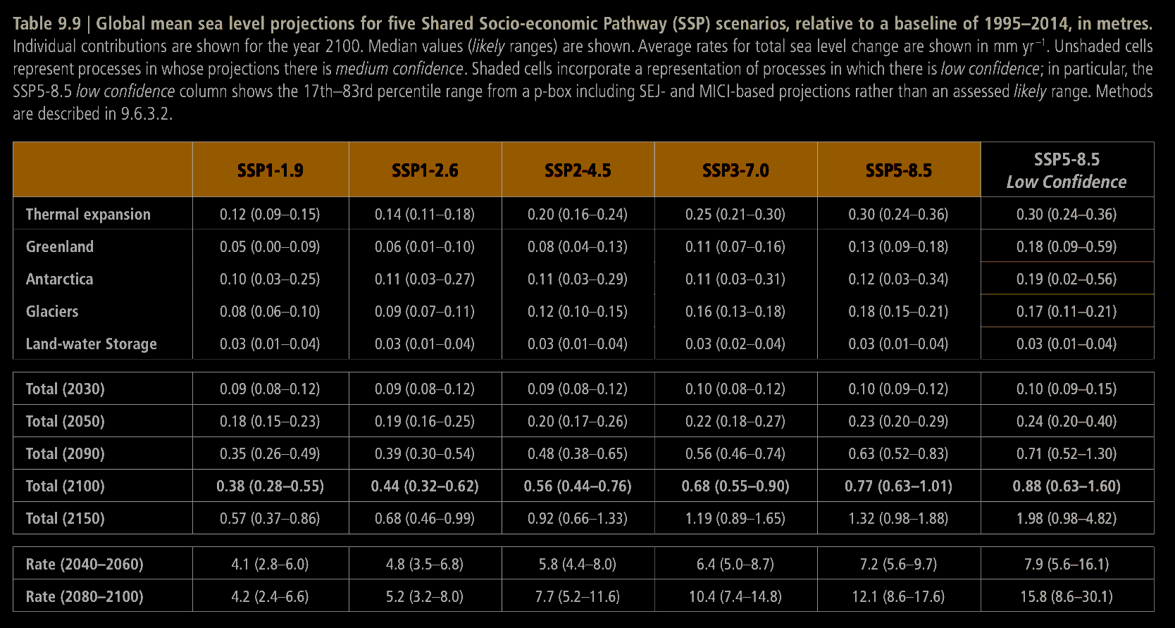
I manually extracted this data into the following table. I'm using the central values they provide, and ignoring the confidence interval. The objective here is just to tell whether the skewed normal fits match up loosely with the expected values. We'll also multiply the values in this dataframe by 1000 to account for the unit difference (our model outputs millimeters, they use meters).

In [48]:

years = [2030, 2050, 2090, 2100, 2150]
values = {
    "126": [0.09, 0.19, 0.39, 0.44, 0.68],
    "245": [0.09, 0.20, 0.48, 0.56, 0.92],
    "585": [0.10, 0.23, 0.63, 0.77, 1.32],
}

val_df = pd.DataFrame(values, index=years)
val_df = val_df * 1000
val_df

years = [2030, 2050, 2090, 2100, 2150] values = { "126": [0.09, 0.19, 0.39, 0.44, 0.68], "245": [0.09, 0.20, 0.48, 0.56, 0.92], "585": [0.10, 0.23, 0.63, 0.77, 1.32], } val_df = pd.DataFrame(values, index=years) val_df = val_df * 1000 val_df

Out[48]:

	126	245	585
2030	90.0	90.0	100.0
2050	190.0	200.0	230.0
2090	390.0	480.0	630.0
2100	440.0	560.0	770.0
2150	680.0	920.0	1320.0

Now we can compare this against our models. We're focusing on the 'medium' confidence scenarios.

We'll try the median, which is what they use, but notably their median is different than ours. Actually I'm not even sure what their median is exactly referring to, but it probably factors in the quantiles somehow, which are ignored here.

In [65]:

scenarios = val_df.columns
diff_df = deepcopy(val_df)
comp_df = deepcopy(val_df)
for scen in scenarios:
    slp = SLP.load(confidence="medium", scenario=scen)
    slp.forecast.train()
    pred = pd.Series([slp.forecast.vmed(year) for year in years], index=years)
    comp_df[f"model_{scen}"] = pred
    diff_df[scen] = (round((pred / diff_df[scen]) - 1, 4)) * 100
diff_df["avg_percent_diff"] = diff_df.mean(axis=1)

scenarios = val_df.columns diff_df = deepcopy(val_df) comp_df = deepcopy(val_df) for scen in scenarios: slp = SLP.load(confidence="medium", scenario=scen) slp.forecast.train() pred = pd.Series([slp.forecast.vmed(year) for year in years], index=years) comp_df[f"model_{scen}"] = pred diff_df[scen] = (round((pred / diff_df[scen]) - 1, 4)) * 100 diff_df["avg_percent_diff"] = diff_df.mean(axis=1)

[SUCCESS] distribution fit with params: a=6.336008526116064, loc=36.217225776201914, scale=26.499101164646206
[SUCCESS] distribution fit with params: a=5.395765778925574, loc=65.96713161669996, scale=51.89790726109507
[SUCCESS] distribution fit with params: a=5.2516139267483695, loc=91.79716693057506, scale=84.3977925731794
[SUCCESS] distribution fit with params: a=5.375537285516717, loc=127.07699100029154, scale=120.50862925192759
[SUCCESS] distribution fit with params: a=4.75210367967559, loc=148.9815539003562, scale=161.9565510001559
[SUCCESS] distribution fit with params: a=4.9794339762155015, loc=181.0611547138783, scale=204.96800639226774
[SUCCESS] distribution fit with params: a=3.7235340713646448, loc=197.14713750731312, scale=259.8152957042531
[SUCCESS] distribution fit with params: a=3.8853618584306986, loc=216.11771757184601, scale=309.2036028951542
[SUCCESS] distribution fit with params: a=3.609209400576966, loc=230.41995592402873, scale=361.2054271926496
[SUCCESS] distribution fit with params: a=6.371515168495243, loc=254.63459928563884, scale=420.5578295282163
[SUCCESS] distribution fit with params: a=6.499318451859498, loc=271.9702126298085, scale=472.8110066298254
[SUCCESS] distribution fit with params: a=6.604161455986308, loc=287.0527075970766, scale=524.7800963533753
[SUCCESS] distribution fit with params: a=6.729952755482406, loc=301.1037168259759, scale=576.8664760591203
[SUCCESS] distribution fit with params: a=6.836750088876363, loc=314.06869887162077, scale=629.1149063926257
[SUCCESS] distribution fit with params: a=5.743975740306972, loc=36.164234604470565, scale=25.648743180786962
[SUCCESS] distribution fit with params: a=5.182231462895766, loc=66.65545648583796, scale=50.66653599973423
[SUCCESS] distribution fit with params: a=4.826670666558719, loc=98.77597705691915, scale=80.71888977645303
[SUCCESS] distribution fit with params: a=6.097923283953435, loc=143.43576407889822, scale=117.52710654937184
[SUCCESS] distribution fit with params: a=4.604312301237858, loc=177.73431558284676, scale=161.17478717133943
[SUCCESS] distribution fit with params: a=4.302638376657248, loc=217.3774712332787, scale=211.59553546919736
[SUCCESS] distribution fit with params: a=4.188282356556575, loc=253.6808747205983, scale=272.53183761119806
[SUCCESS] distribution fit with params: a=4.250054124385981, loc=289.71291494458524, scale=338.9957902267304
[SUCCESS] distribution fit with params: a=4.281880127311123, loc=328.98451633078946, scale=406.535462481623
[SUCCESS] distribution fit with params: a=6.673061154188609, loc=350.57018541954324, scale=490.7650896090627
[SUCCESS] distribution fit with params: a=6.75855006960453, loc=384.72780117768656, scale=560.9933986515815
[SUCCESS] distribution fit with params: a=6.787120353791238, loc=417.6704656895899, scale=631.2479293880192
[SUCCESS] distribution fit with params: a=6.8403784471332525, loc=449.7551450384476, scale=701.49002417919
[SUCCESS] distribution fit with params: a=6.881719567282601, loc=480.77103780606205, scale=771.0365584054249
[SUCCESS] distribution fit with params: a=6.35241015973173, loc=35.99658069718064, scale=28.111580396222273
[SUCCESS] distribution fit with params: a=5.096871305510005, loc=70.66973343458793, scale=54.96140440412516
[SUCCESS] distribution fit with params: a=5.763663587377232, loc=110.74874004286636, scale=89.83310367254231
[SUCCESS] distribution fit with params: a=5.228228021043594, loc=163.5534544090983, scale=133.38997146068937
[SUCCESS] distribution fit with params: a=5.101378964357277, loc=213.72709579057965, scale=186.94999434641414
[SUCCESS] distribution fit with params: a=5.636522073675502, loc=274.8963368738746, scale=251.0756454178623
[SUCCESS] distribution fit with params: a=4.782617220601494, loc=334.7672629463968, scale=331.61832359032053
[SUCCESS] distribution fit with params: a=5.308169643484584, loc=414.5584482139646, scale=416.1315973696705
[SUCCESS] distribution fit with params: a=5.22946285210722, loc=489.93843964346445, scale=523.6084467375629
[SUCCESS] distribution fit with params: a=6.757180784739575, loc=492.1731895549258, scale=658.6826221257295
[SUCCESS] distribution fit with params: a=6.732781229967694, loc=557.3925777094735, scale=762.216229241717
[SUCCESS] distribution fit with params: a=6.769984719450592, loc=619.7033640925753, scale=864.7711249649267
[SUCCESS] distribution fit with params: a=6.862736894866174, loc=677.0954078594514, scale=968.2556837673278
[SUCCESS] distribution fit with params: a=6.979824091070947, loc=729.4440840890079, scale=1071.8957799258405

In [68]:

comp_df

comp_df

Out[68]:

	126	245	585	model_126	model_245	model_585
2030	90.0	90.0	100.0	100.971427	100.828952	107.739857
2050	190.0	200.0	230.0	208.358061	222.706512	253.522322
2090	390.0	480.0	630.0	424.568615	518.315754	695.231726
2100	440.0	560.0	770.0	473.816901	603.137238	843.101882
2150	680.0	920.0	1320.0	738.400219	1000.827256	1452.426764

In [69]:

diff_df

diff_df

Out[69]:

	126	245	585	avg_percent_diff
2030	12.19	12.03	7.74	10.653333
2050	9.66	11.35	10.23	10.413333
2090	8.86	7.98	10.35	9.063333
2100	7.69	7.70	9.49	8.293333
2150	8.59	8.79	10.03	9.136667

We can rerun this with the midpoint.

In [70]:

scenarios = val_df.columns
diff_df = deepcopy(val_df)
comp_df = deepcopy(val_df)
for scen in scenarios:
    slp = SLP.load(confidence="medium", scenario=scen)
    slp.forecast.train()
    pred = pd.Series([slp.forecast.vmid(year) for year in years], index=years)
    comp_df[f"model_{scen}"] = pred
    diff_df[scen] = (round((pred / diff_df[scen]) - 1, 4)) * 100
diff_df["avg_percent_diff"] = diff_df.mean(axis=1)

scenarios = val_df.columns diff_df = deepcopy(val_df) comp_df = deepcopy(val_df) for scen in scenarios: slp = SLP.load(confidence="medium", scenario=scen) slp.forecast.train() pred = pd.Series([slp.forecast.vmid(year) for year in years], index=years) comp_df[f"model_{scen}"] = pred diff_df[scen] = (round((pred / diff_df[scen]) - 1, 4)) * 100 diff_df["avg_percent_diff"] = diff_df.mean(axis=1)

[SUCCESS] distribution fit with params: a=6.336008526116064, loc=36.217225776201914, scale=26.499101164646206
[SUCCESS] distribution fit with params: a=5.395765778925574, loc=65.96713161669996, scale=51.89790726109507
[SUCCESS] distribution fit with params: a=5.2516139267483695, loc=91.79716693057506, scale=84.3977925731794
[SUCCESS] distribution fit with params: a=5.375537285516717, loc=127.07699100029154, scale=120.50862925192759
[SUCCESS] distribution fit with params: a=4.75210367967559, loc=148.9815539003562, scale=161.9565510001559
[SUCCESS] distribution fit with params: a=4.9794339762155015, loc=181.0611547138783, scale=204.96800639226774
[SUCCESS] distribution fit with params: a=3.7235340713646448, loc=197.14713750731312, scale=259.8152957042531
[SUCCESS] distribution fit with params: a=3.8853618584306986, loc=216.11771757184601, scale=309.2036028951542
[SUCCESS] distribution fit with params: a=3.609209400576966, loc=230.41995592402873, scale=361.2054271926496
[SUCCESS] distribution fit with params: a=6.371515168495243, loc=254.63459928563884, scale=420.5578295282163
[SUCCESS] distribution fit with params: a=6.499318451859498, loc=271.9702126298085, scale=472.8110066298254
[SUCCESS] distribution fit with params: a=6.604161455986308, loc=287.0527075970766, scale=524.7800963533753
[SUCCESS] distribution fit with params: a=6.729952755482406, loc=301.1037168259759, scale=576.8664760591203
[SUCCESS] distribution fit with params: a=6.836750088876363, loc=314.06869887162077, scale=629.1149063926257
[SUCCESS] distribution fit with params: a=5.743975740306972, loc=36.164234604470565, scale=25.648743180786962
[SUCCESS] distribution fit with params: a=5.182231462895766, loc=66.65545648583796, scale=50.66653599973423
[SUCCESS] distribution fit with params: a=4.826670666558719, loc=98.77597705691915, scale=80.71888977645303
[SUCCESS] distribution fit with params: a=6.097923283953435, loc=143.43576407889822, scale=117.52710654937184
[SUCCESS] distribution fit with params: a=4.604312301237858, loc=177.73431558284676, scale=161.17478717133943
[SUCCESS] distribution fit with params: a=4.302638376657248, loc=217.3774712332787, scale=211.59553546919736
[SUCCESS] distribution fit with params: a=4.188282356556575, loc=253.6808747205983, scale=272.53183761119806
[SUCCESS] distribution fit with params: a=4.250054124385981, loc=289.71291494458524, scale=338.9957902267304
[SUCCESS] distribution fit with params: a=4.281880127311123, loc=328.98451633078946, scale=406.535462481623
[SUCCESS] distribution fit with params: a=6.673061154188609, loc=350.57018541954324, scale=490.7650896090627
[SUCCESS] distribution fit with params: a=6.75855006960453, loc=384.72780117768656, scale=560.9933986515815
[SUCCESS] distribution fit with params: a=6.787120353791238, loc=417.6704656895899, scale=631.2479293880192
[SUCCESS] distribution fit with params: a=6.8403784471332525, loc=449.7551450384476, scale=701.49002417919
[SUCCESS] distribution fit with params: a=6.881719567282601, loc=480.77103780606205, scale=771.0365584054249
[SUCCESS] distribution fit with params: a=6.35241015973173, loc=35.99658069718064, scale=28.111580396222273
[SUCCESS] distribution fit with params: a=5.096871305510005, loc=70.66973343458793, scale=54.96140440412516
[SUCCESS] distribution fit with params: a=5.763663587377232, loc=110.74874004286636, scale=89.83310367254231
[SUCCESS] distribution fit with params: a=5.228228021043594, loc=163.5534544090983, scale=133.38997146068937
[SUCCESS] distribution fit with params: a=5.101378964357277, loc=213.72709579057965, scale=186.94999434641414
[SUCCESS] distribution fit with params: a=5.636522073675502, loc=274.8963368738746, scale=251.0756454178623
[SUCCESS] distribution fit with params: a=4.782617220601494, loc=334.7672629463968, scale=331.61832359032053
[SUCCESS] distribution fit with params: a=5.308169643484584, loc=414.5584482139646, scale=416.1315973696705
[SUCCESS] distribution fit with params: a=5.22946285210722, loc=489.93843964346445, scale=523.6084467375629
[SUCCESS] distribution fit with params: a=6.757180784739575, loc=492.1731895549258, scale=658.6826221257295
[SUCCESS] distribution fit with params: a=6.732781229967694, loc=557.3925777094735, scale=762.216229241717
[SUCCESS] distribution fit with params: a=6.769984719450592, loc=619.7033640925753, scale=864.7711249649267
[SUCCESS] distribution fit with params: a=6.862736894866174, loc=677.0954078594514, scale=968.2556837673278
[SUCCESS] distribution fit with params: a=6.979824091070947, loc=729.4440840890079, scale=1071.8957799258405

In [72]:

comp_df

comp_df

Out[72]:

	126	245	585	model_126	model_245	model_585
2030	90.0	90.0	100.0	95.528640	95.699737	102.257837
2050	190.0	200.0	230.0	195.760647	209.078618	239.912564
2090	390.0	480.0	630.0	400.967678	489.904611	652.204921
2100	440.0	560.0	770.0	448.375494	568.807158	789.667120
2150	680.0	920.0	1320.0	658.970697	903.027626	1315.112348

In [73]:

diff_df

diff_df

Out[73]:

	126	245	585	avg_percent_diff
2030	6.14	6.33	2.26	4.910000
2050	3.03	4.54	4.31	3.960000
2090	2.81	2.06	3.52	2.796667
2100	1.90	1.57	2.55	2.006667
2150	-3.09	-1.84	-0.37	-1.766667

The midpoint seems to work much better at matching the figures they provide. Either way, the skewed normal distribution models fit to just the sea level change data (represented as a distribution and ignoring quantiles) for each decade pretty well. Going from this fairly non-rigorous and unscientific eyeballing of the model outputs and the IPCC figures, they are usable, with somewhere maybe in the range of 5-10% error, acceptable for this project.